This article provides a closer look at Kyber, now standardized as ML-KEM, which is based on the Module Learning with Errors problem. The first part introduces the required operations, namely addition and multiplication within a polynomial ring. The second part then examines the encapsulation and decapsulation steps in detail, one step at a time. The article concludes with an analysis of the scheme’s correctness.

Operations

In Kyber, the fundamental operations are performed using polynomials. Whether we are dealing with a scalar, a matrix, or a vector, every component consists of a polynomial. Such a polynomial might look like this, for example:

To reduce the amount of notation required, we can also represent it as a table:

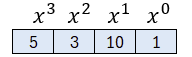
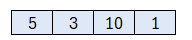
Since the powers in the header always increase from right to left and remain the same, we can simplify this further into a list or 4-tuple:

Before looking at the addition of two polynomials, we first need to establish that all operations in Kyber are performed modulo a prime number p. This is therefore directly analogous to the simplified version, in which we also reduced all values modulo p. This applies to all coefficients of the polynomials as well: if a coefficient has a value greater than or equal to p, we can immediately reduce it modulo p. Here and throughout the following sections, we will use (p=17). Every sum and every product is therefore calculated modulo 17.

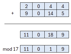
Let us take a look at addition. The coefficients are added together, just as one would expect even without any knowledge of polynomials. The result is then reduced modulo p, which in our case means modulo 17. We therefore obtain coefficients from the interval ([0,p)).

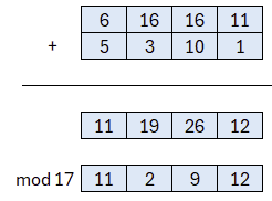
For a better understanding, here is another calculation example:

Multiplication, on the other hand, is somewhat more difficult than addition. It begins in a way that is very similar to standard long multiplication and is easy to understand. However, we need to ensure that the polynomials do not become longer, because all polynomials in Kyber have a fixed length. In our example, the degree is 3, meaning that we have a total of four coefficients, corresponding to the powers from 0 to 3. In the „real“ Kyber, the degree is 255, meaning that we have to work with 256 coefficients. As is well known, however, the result of a multiplication—the product—is often considerably larger than the original factors. For this reason, the multiplication is performed first, after which the result is reduced again using polynomial division in order to return to the fixed length of 4 coefficients, or 256 coefficients in Kyber.

We will begin with the multiplication using a simple example.

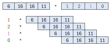
As mentioned, the first step resembles the standard long-multiplication method: we perform the multiplication and examine the result.

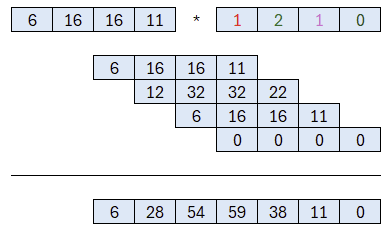
Just as with addition, we need to reduce the coefficients in the result modulo (p).

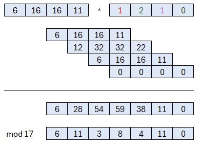
This gives us a polynomial of degree 6. Just so that we do not forget that we are dealing with polynomials, I would like to present the result once again in this form:

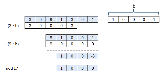
However, this product, the result of multiplying two polynomials of degree 3 and therefore a polynomial of degree 6, is too long. In Kyber, all polynomials have the same length. For this reason, we need to reduce the result using polynomial division. A specific polynomial is used for this purpose: in Kyber, this polynomial is (x²⁵⁶+1). Here, in our example, we use (b=x⁴+1). We represent it in binary form as follows:

This polynomial (b) is intentionally not colored blue so that it can be distinguished more easily from the other polynomials. All products, that is, all results of multiplications, are divided by this polynomial. The quotient is not important to us; only the remainder is of interest. We therefore multiply the coefficients of (b) by an appropriate value and subtract the result from our polynomial. This value is determined by the leading coefficient. At the end, the result must be reduced modulo (p), which in this case means modulo 17.

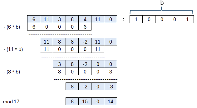
The result is therefore:

For a better understanding, here is another example:

In this way, we can convert all multiplication results back into the four-element form. This also completes the description of all the required operations. Provided that the explanations of addition and multiplication were understandable, we now know all the essential tools required for Kyber.

Key Generation

In Kyber, the public key consists of a matrix A and a vector t.

However, it must be taken into account that the components of the matrices and vectors are themselves polynomials. In this example, A is therefore a 2 x 2 matrix containing four polynomials, while t is a vector containing two polynomials. We will now determine A and t step by step.

Let us first consider the 2 x 2 matrix A. In Kyber, this matrix is chosen at random. More precisely, it is generated deterministically from a 256-bit random seed. This reduces the amount of key material that needs to be transmitted. In our example, we simply fill the polynomials with random coefficients smaller than p.

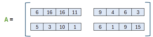
We have now defined (or randomly chosen) A. The vector t is obtained by multiplying A by s and then adding e. Before determining t, let us therefore first take a look at s and e.

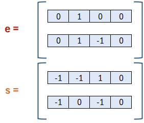
Like the matrix A, the vectors e and s can be chosen freely. For e, it is important that only small coefficients, values close to zero, are selected. This is not quite as important for s, but the scheme does not become less secure if we do the same here. For this reason, values close to zero were chosen for both vectors. Strictly speaking, -1 corresponds to 16, since -1 mod 17 = 16. However, writing -1 makes it clearer that the coefficients are close to zero. The vector t is now calculated from these coefficients:

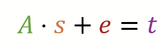
Thus, A is multiplied by s, and e is added to the result. All intermediate and final results can always be reduced modulo q, which in this case means modulo 17.

Matrix-vector multiplication is performed in exactly the same way as in linear algebra. The only difference is that the polynomial multiplication and addition operations defined above are used.

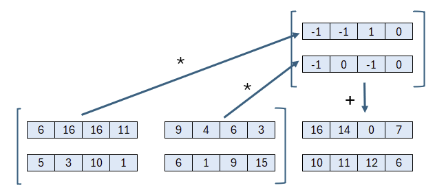
The first component of the resulting vector is therefore calculated as follows:

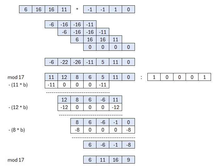
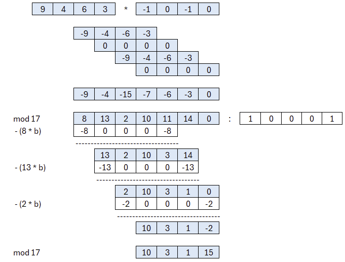
Anyone wondering how this result is obtained can now take a closer look at the two multiplications and the subsequent addition.

First Multiplication with Polynomial Division

Second Multiplication with Polynomial Division

Addition

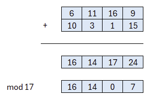
This is how the resulting vector A * s is calculated. To continue, the result is added to e, the error vector:

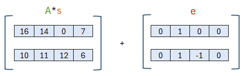
This gives us the second component of our public key.

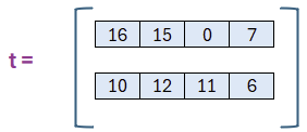
At this point, it is probably worth briefly reviewing what we have done. A randomly generated but publicly known matrix A was multiplied by a vector s, after which a vector e was added to the result. The vector s is the private key. If we only formed the product of A and s, the operation could be reversed using Gaussian elimination. However, we also add an error vector e. Recovering the private key would therefore require reversing the operation while accounting for random error vectors. This is assumed to be computationally difficult even for quantum computers.

We have now generated our public key. It consists of the matrix A and the vector t and can be transmitted to the sender. In our example, the sender is the person who wants to transmit a message, while the recipient is the person who will subsequently decrypt it. The recipient therefore generates the key material and sends the public key to the sender.

Encapsulation

We have now successfully generated the key material. In the following, the sender will perform a key encapsulation and generate two ciphertext components: u and v. Although the simplified example below uses a bit sequence m to illustrate the underlying mathematical operations, Kyber is not used to encrypt an arbitrary message directly. Instead, it encapsulates a shared secret, which can subsequently be used with a symmetric encryption algorithm to encrypt the actual message.

We do not yet know what u and v will look like. However, it is probably already possible to guess that one of these components will contain information derived from m. Spoiler alert: v contains the encoded value, while u enables the recipient to recover it using the private key s.

Before we examine u and v, we first need to talk about the encoded value m. In our simplified example, m consists of the bits 0 and 1. For example, if we use the bits 1011, we can represent them as a polynomial:

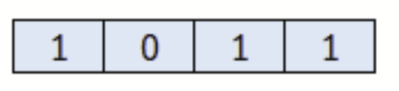
To process m in Kyber, it must first be scaled. Scaling means multiplying it by (p/2), which in this case is (17/2), and then rounding up. In our example, we therefore replace every 1 with a 9, while leaving the zeros unchanged.

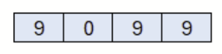
This is m, scaled by (p/2). Whenever m is mentioned in the following, it refers to this scaled sequence. This scaling is necessary because the recovery process is not lossless at the level of the polynomial coefficients. After decapsulation, the values will no longer necessarily be exactly 9099 as they are here, but may differ slightly, for example, they might be 8179. In that case, however, the original sequence 9099 can still be recovered quite easily, because every 7 or 8 is closer to 9, while every (-1), 0, or 1 is closer to 0.

We therefore define m as this scaled value.

For the remainder of the encapsulation process, we require a vector r, a vector e₁, and a scalar e₂, all containing random values. However, just as with e and s above, their coefficients should be small, for example, 1, 2, or 3 in this simplified example. To make this absolutely clear once again: these values are chosen at random, and we could choose different values without causing any problems!

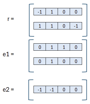
We are now ready to take a closer look at u and v. Let us begin with u.

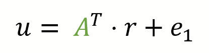
The superscript T denotes the transposed matrix. Transposing means reflecting the matrix across its main diagonal: rows become columns, and columns become rows. Let us take a look:

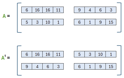
The main diagonal remains unchanged, and only two polynomials exchange positions. In the next step, we can determine u through multiplication and addition, with all operations performed modulo q.

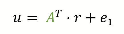
To calculate u, we therefore transpose the already known matrix A, multiply it by the random vector r, and add e₁. In case it was not immediately apparent, the same underlying construction appears once again in u, only with new values. It is therefore used both to generate the public key and here during encapsulation.

Now let us take a closer look at the second component, v:

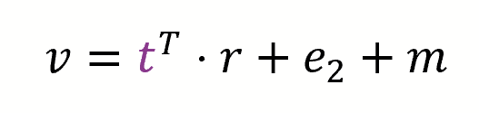
In this case, it is not a matrix that is transposed, but a vector. Previously, t had two rows and one column. After transposition, t therefore has one row and two columns. This also defines the scalar product with r. As always, however, the result is a polynomial. Finally, e₂ and m are added.

We have now successfully encapsulated the value represented by m=1011 and obtained the six values that form the ciphertext. Both components are required for decapsulation: u and v.

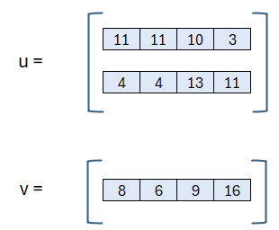
These values can now be transmitted to the recipient.

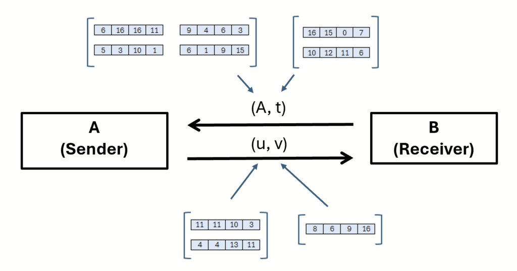
Once u and v have successfully arrived at the recipient, we can begin the decapsulation process.

Decapsulation

While encapsulation requires a certain amount of work, recovering the encoded value during decapsulation is comparatively straightforward. Here, m_new is the result of this recovery step. It will become clear later why it is called m_new rather than simply m.

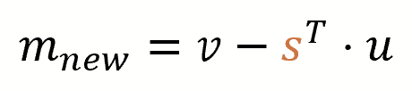
We transpose our secret key s, multiply it by the vector u received from the sender, and subtract the result from v.

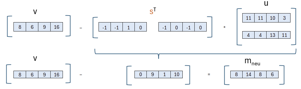
Only by transposing s can we calculate the required product of the polynomials. But does simply transposing it not break something? No, because v also contains the transposed vector t, and the transposed t implicitly contains the correspondingly transposed s. This will be explained in greater detail in the section on correctness.

We have now successfully recovered the transmitted value.

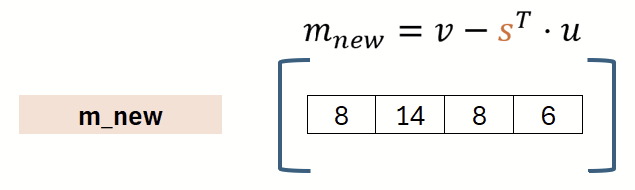
But what is this? The result m_new = 8, 14, 8, 6 differs from the original value m=1, 0, 1, 1. Does that mean everything is wrong? No! This is correct and expected. After all, r, e, e₁, and e₂ introduce several „errors“ into the calculation, not all of which can be completely removed at the end. However, we deliberately chose small coefficients for these errors. We therefore expect the result to shift only slightly. At the level of the polynomial coefficients, Kyber does not reproduce the exact values that were originally used. Nevertheless, because each result is either closer to the encoding of 0 or to the encoding of 1, we can reconstruct the original bit.

If we evaluate the values 8, 14, 8, and 6 according to their distance from 0 and 9, we conclude that 8 was most likely a 9, that 14 was most likely a 0, and that 6 is also relatively close to 9. With the small prime p used here, namely 17, these distinctions are admittedly quite narrow. The original scheme uses a larger modulus, (q=3329), which makes the result less ambiguous. However, even in the original scheme, decapsulation can fail if the values of e, s, e₁, and e₂ are particularly unfavorable. The protocol accounts for this possibility.

Correctness

The best way to understand why the scheme works correctly is to begin at the end and substitute the variables in reverse order. We therefore start with the decapsulation equation and replace u and v with the expressions used to calculate them earlier.

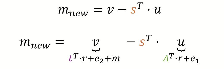
We are not quite finished yet, because t, which is contained in v, was itself calculated from A, s, and e at the very beginning:

We now fully substitute v and u and examine the resulting expression without losing track of its individual parts.

The question is now which parts of this expression can be simplified. First, we can look at the algebraic rules for transposed matrices. In brief:

• (A + B)^T = A^T + B^T
• (A * B)^T = B^T * A^T

Using these rules, we can easily transform the first set of parentheses, which represents the original t:

Next, we can expand this expression by multiplying it by the adjacent r.

Now let us examine the right-hand side. Remember to take the minus sign in front of s into account!

We therefore expand the right-hand side in the usual way.

Now that the expansion is complete, we can remove all parentheses and examine the result.

That is quite a lot of terms. However, just as in school algebra, we can simply check whether the same product appears twice with opposite signs. Fortunately, that is exactly what happens!

We can therefore see that all terms involving the matrix A cancel out completely. At the same time, however, it also becomes clear that several terms remain. Let us consider whether any of these remaining terms can be eliminated as well.

As a reminder, e was chosen by the recipient, but r originates from the sender. The value e₂ also comes from the sender and therefore cannot be removed by the recipient. Although the recipient knows the private key s, e₁ was chosen by the sender and is therefore unknown. The colors make it easy to see that, as the recipient, we cannot simplify the expression any further. We are therefore finished.

At this point, it should become clear why small coefficients were chosen for the error terms e, e₁, and e₂, as well as for r. These terms remain in the result after decapsulation and cannot be removed completely. In an extreme case, this can indeed cause the encoded value to be recovered incorrectly. However, the scheme is designed to account for this possibility, and such a failure should occur only rarely.

Further Information

At this point, I would also like to highlight the excellent explanations provided by Ruben Gonzalez, whose example values are used throughout this article as well. Of course, I would also like to refer readers to the original paper.

Finally, I would like to make the Kyber implementation in Excel available here. The example presented above can be followed in full within this document.

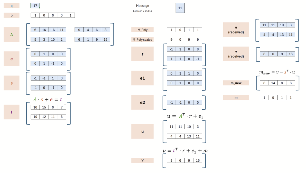
No macros were used. However, due to the use of LAMBDA functions, the implementation will only work with Microsoft 365 or Excel 2024.

_{SHA256: F64A011F6AC20233836C4FFFFB362014F564A51FD8FB466224D568C72127E8B9}